Chapter 2
The Insurance Market and Our Case Studies.
- Basic statistics by line.
- Density plots.
- Bivariate distributions.
| view | Gross | Net | ||||
|---|---|---|---|---|---|---|
| line | A | B | Total | A | B | Total |
| statistic | ||||||
| Mean | 50.000 | 50.000 | 100.000 | 50.000 | 49.084 | 99.084 |
| CV | 0.100 | 0.150 | 0.090 | 0.100 | 0.123 | 0.079 |
| Skewness | 0.200 | 0.300 | 0.207 | 0.200 | -0.484 | -0.169 |
| Kurtosis | 0.060 | 0.135 | 0.070 | 0.060 | -0.474 | -0.157 |


Chapter 4
Measuring Risk with Quantiles, VaR, and TVaR.
- VaR, TVaR, and EPD plots and statistics.

| view | Gross | Net | ||||||||
|---|---|---|---|---|---|---|---|---|---|---|
| line | A | B | Benefit | Sum | Total | A | B | Benefit | Sum | Total |
| statistic | ||||||||||
| VaR 90.0 | 56 | 60 | 0.041 | 116 | 112 | 56 | 56 | 0.0344 | 113 | 109 |
| VaR 95.0 | 58 | 63 | 0.053 | 121 | 115 | 58 | 56 | 0.0296 | 115 | 111 |
| VaR 97.5 | 60 | 66 | 0.063 | 126 | 119 | 60 | 56 | 0.026 | 116 | 113 |
| VaR 99.0 | 62 | 69 | 0.0743 | 131 | 122 | 62 | 56 | 0.0224 | 119 | 116 |
| VaR 99.6 | 64 | 72 | 0.0843 | 136 | 126 | 64 | 59 | 0.0452 | 124 | 118 |
| VaR 99.9 | 67 | 76 | 0.0974 | 143 | 131 | 67 | 64 | 0.0754 | 130 | 121 |
| TVaR 90.0 | 59 | 64 | 0.0568 | 123 | 117 | 59 | 58 | 0.0444 | 117 | 112 |
| TVaR 95.0 | 61 | 67 | 0.0664 | 128 | 120 | 61 | 59 | 0.0477 | 120 | 114 |
| TVaR 97.5 | 62 | 69 | 0.075 | 132 | 123 | 62 | 59 | 0.048 | 122 | 116 |
| TVaR 99.0 | 64 | 72 | 0.0849 | 137 | 126 | 64 | 59 | 0.0464 | 124 | 118 |
| TVaR 99.6 | 66 | 75 | 0.0938 | 141 | 129 | 66 | 62 | 0.0666 | 128 | 120 |
| TVaR 99.9 | 69 | 79 | 0.106 | 148 | 134 | 69 | 66 | 0.0931 | 135 | 123 |
| EPD 10.0 | 45 | 46 | 0.0146 | 92 | 91 | 45 | 45 | 0.0122 | 91 | 90 |
| EPD 5.0 | 49 | 51 | 0.0277 | 100 | 97 | 49 | 49 | 0.0232 | 98 | 96 |
| EPD 2.5 | 52 | 55 | 0.0397 | 107 | 103 | 52 | 52 | 0.0323 | 104 | 101 |
| EPD 1.0 | 55 | 59 | 0.0536 | 114 | 108 | 55 | 54 | 0.0392 | 109 | 105 |
| EPD 0.4 | 57 | 63 | 0.0656 | 120 | 113 | 57 | 55 | 0.0407 | 113 | 108 |
| EPD 0.1 | 60 | 68 | 0.081 | 128 | 119 | 60 | 56 | 0.0374 | 117 | 112 |
Chapter 7
Guide to the Practice Chapters.
- Summary of pricing by unit.
- Specification of ceded reinsurance.
| portfolio | Gross | Net |
|---|---|---|
| stat | ||
| Loss | 100 | 99.08 |
| Margin | 3.423 | 2.464 |
| Premium | 103.4 | 101.5 |
| Loss Ratio | 0.967 | 0.976 |
| Capital | 34.23 | 24.64 |
| Rate of Return | 0.1 | 0.1 |
| Assets | 137.7 | 126.2 |
| Leverage | 3.021 | 4.121 |
| Tame | |
|---|---|
| item | |
| Reinsured Line | B |
| Reinsurance Type | Aggregate |
| Attachment Probability | 0.2 |
| Attachment | 56.17 |
| Exhaustion Probability | 0.01 |
| Limit | 12.91 |
Chapter 9
Classical Portfolio Pricing Practice.
- Classical pricing stand-alone by unit and in total, with parameters.
- Impact of diversification: sum of stand-alone premiums compared to portfolio premium.
- Stand-alone vs. diversified loss ratios.
- Stand-alone vs. diversified loss, premium, and capital for CCoC pricing.
- Stand-alone vs. diversified all insurance statistics for CCoC pricing.
| Parameters | A | B | Total | ||||
|---|---|---|---|---|---|---|---|
| Value | Gross | Net | Gross | Net | Gross | Ceded | |
| method | |||||||
| Net | 50.000 | 49.084 | 50.000 | 99.084 | 100.000 | 0.916 | |
| Expected Value | 0.034 | 51.712 | 50.765 | 51.712 | 102.476 | 103.423 | 0.947 |
| Variance | 0.042 | 51.053 | 50.620 | 52.370 | 101.673 | 103.423 | 1.750 |
| Esscher | 0.041 | 51.034 | 50.468 | 52.389 | 101.503 | 103.423 | 1.920 |
| Exponential | 0.080 | 51.028 | 50.420 | 52.395 | 101.447 | 103.423 | 1.976 |
| Semi-Variance | 0.080 | 51.051 | 50.330 | 52.425 | 101.411 | 103.423 | 2.012 |
| VaR | 0.659 | 51.906 | 52.750 | 52.750 | 102.672 | 103.422 | 0.750 |
| Dutch | 0.953 | 51.899 | 51.498 | 52.846 | 102.096 | 103.423 | 1.327 |
| Standard Deviation | 0.380 | 51.899 | 51.377 | 52.848 | 102.061 | 103.423 | 1.362 |
| Fischer | 0.523 | 51.897 | 51.149 | 52.881 | 101.907 | 103.423 | 1.516 |
| Total | SoP | Delta | ||||
|---|---|---|---|---|---|---|
| Gross | Net | Gross | Net | Gross | Net | |
| method | ||||||
| Net | 100.000 | 99.084 | 100.000 | 99.084 | 0.000 | 0.000 |
| Expected Value | 103.423 | 102.476 | 103.423 | 102.476 | 0.000 | 0.000 |
| Variance | 103.423 | 101.673 | 103.423 | 101.673 | -0.000 | -0.000 |
| Esscher | 103.423 | 101.503 | 103.423 | 101.503 | 0.000 | 0.000 |
| Exponential | 103.423 | 101.447 | 103.423 | 101.447 | 0.000 | 0.000 |
| Semi-Variance | 103.423 | 101.411 | 103.477 | 101.382 | 0.054 | -0.029 |
| VaR | 103.422 | 102.672 | 104.656 | 104.656 | 1.234 | 1.984 |
| Dutch | 103.423 | 102.096 | 104.745 | 103.397 | 1.322 | 1.301 |
| Standard Deviation | 103.423 | 102.061 | 104.747 | 103.276 | 1.324 | 1.215 |
| Fischer | 103.423 | 101.907 | 104.778 | 103.047 | 1.355 | 1.140 |
| A | B | Total | ||||
|---|---|---|---|---|---|---|
| Gross | Net | Gross | Net | Gross | Ceded | |
| method | ||||||
| Net | 1 | 1 | 1 | 1 | 1 | 1 |
| Expected Value | 0.967 | 0.967 | 0.967 | 0.967 | 0.967 | 0.967 |
| Variance | 0.979 | 0.97 | 0.955 | 0.975 | 0.967 | 0.523 |
| Esscher | 0.98 | 0.973 | 0.954 | 0.976 | 0.967 | 0.477 |
| Exponential | 0.98 | 0.974 | 0.954 | 0.977 | 0.967 | 0.463 |
| Semi-Variance | 0.979 | 0.975 | 0.954 | 0.977 | 0.967 | 0.455 |
| VaR | 0.963 | 0.931 | 0.948 | 0.965 | 0.967 | 1.22 |
| Dutch | 0.963 | 0.953 | 0.946 | 0.97 | 0.967 | 0.69 |
| Standard Deviation | 0.963 | 0.955 | 0.946 | 0.971 | 0.967 | 0.672 |
| Fischer | 0.963 | 0.96 | 0.946 | 0.972 | 0.967 | 0.604 |
| Gross SoP | Gross Total | Gross Redn | Net SoP | Net Total | Net Redn | ||
|---|---|---|---|---|---|---|---|
| method | statistic | ||||||
| No Default | Loss | 100 | 100 | -0.0% | 99.08 | 99.08 | -0.0% |
| Premium | 104.9 | 103.4 | -1.4% | 102.9 | 101.5 | -1.3% | |
| Capital | 48.69 | 34.23 | -29.7% | 37.79 | 24.64 | -34.8% | |
| With Default | Loss | 100 | 100 | 0.0% | 99.08 | 99.08 | 0.0% |
| Premium | 104.9 | 103.4 | -1.4% | 102.9 | 101.5 | -1.3% | |
| Capital | 48.69 | 34.23 | -29.7% | 37.79 | 24.64 | -34.8% |
| portfolio | Gross | Net | ||||||
|---|---|---|---|---|---|---|---|---|
| line | A | B | SoP | Total | A | SoP | Total | |
| method | statistic | |||||||
| No Default | Loss | 50 | 50 | 100 | 100 | 50 | 99.08 | 99.08 |
| Margin | 1.888 | 2.982 | 4.869 | 3.423 | 1.888 | 3.779 | 2.464 | |
| Premium | 51.89 | 52.98 | 104.9 | 103.4 | 51.89 | 102.9 | 101.5 | |
| Loss Ratio | 0.964 | 0.944 | 0.954 | 0.967 | 0.964 | 0.963 | 0.976 | |
| Capital | 18.88 | 29.82 | 48.69 | 34.23 | 18.88 | 37.79 | 24.64 | |
| Rate of Return | 0.1 | 0.1 | 0.1 | 0.1 | 0.1 | 0.1 | 0.1 | |
| Leverage | 2.749 | 1.777 | 2.154 | 3.021 | 2.749 | 2.722 | 4.121 | |
| Assets | 70.77 | 82.8 | 153.6 | 137.7 | 70.77 | 140.7 | 126.2 | |
| With Default | Loss | 50 | 50 | 100 | 100 | 50 | 99.08 | 99.08 |
| Margin | 1.888 | 2.982 | 4.869 | 3.423 | 1.888 | 3.779 | 2.464 | |
| Premium | 51.89 | 52.98 | 104.9 | 103.4 | 51.89 | 102.9 | 101.5 | |
| Loss Ratio | 0.964 | 0.944 | 0.954 | 0.967 | 0.964 | 0.963 | 0.976 | |
| Capital | 18.88 | 29.82 | 48.69 | 34.23 | 18.88 | 37.79 | 24.64 | |
| Rate of Return | 0.1 | 0.1 | 0.1 | 0.1 | 0.1 | 0.1 | 0.1 | |
| Leverage | 2.749 | 1.777 | 2.154 | 3.021 | 2.749 | 2.722 | 4.121 | |
| Assets | 70.77 | 82.8 | 153.6 | 137.7 | 70.77 | 140.7 | 126.2 | |
Chapter 11
Modern Portfolio Pricing Practice.
- Distortion envelopes based on gross pricing.
- Distortion parameter estimates calibrated to gross pricing.
- Distortion, loss ratio, markup, margin, discount and premium leverage for PH, Wang, Dual, TVaR and CCoC.
- Distortion, loss ratio, markup, margin, discount and premium leverage for PH, Wang, Dual, TVaR, CCoC, and Blend.
- Insurance statistics by asset level for CCoC, PH, Dual, and TVaR distortions.
- Stand-alone pricing and insurance statistics, gross and net, by unit by distortion.

| Param | Error | $P$ | $K$ | Rate of Return | $S$ | |
|---|---|---|---|---|---|---|
| method | ||||||
| ROE | 0.1 | 0 | 103.4 | 34.23 | 0.1 | 99.957u |
| PH | 0.683 | 7.920n | 103.4 | 34.23 | 0.1 | 99.957u |
| Wang | 0.375 | 3.396p | 103.4 | 34.23 | 0.1 | 99.957u |
| Dual | 1.576 | -5.063u | 103.4 | 34.23 | 0.1 | 99.957u |
| Tvar | 0.227 | 9.164u | 103.4 | 34.23 | 0.1 | 99.957u |


| portfolio | Gross | Net | ||||||
|---|---|---|---|---|---|---|---|---|
| line | A | B | SoP | Total | B | SoP | Total | |
| statistic | distortion | |||||||
| Loss | CCoC | 50 | 50 | 100 | 100 | 49.08 | 99.08 | 99.08 |
| Margin | CCoC | 1.888 | 2.982 | 4.869 | 3.423 | 1.891 | 3.779 | 2.464 |
| PH | 1.896 | 2.891 | 4.787 | 3.423 | 1.822 | 3.718 | 2.765 | |
| Wang | 1.898 | 2.861 | 4.759 | 3.423 | 2.09 | 3.988 | 2.904 | |
| Dual | 1.9 | 2.835 | 4.735 | 3.423 | 2.355 | 4.255 | 3.03 | |
| TVaR | 1.901 | 2.81 | 4.711 | 3.423 | 2.541 | 4.442 | 3.155 | |
| Blend | 1.9 | 2.959 | 4.859 | 3.438 | 1.621 | 3.521 | 2.562 | |
| Premium | CCoC | 51.89 | 52.98 | 104.9 | 103.4 | 50.98 | 102.9 | 101.5 |
| PH | 51.9 | 52.89 | 104.8 | 103.4 | 50.91 | 102.8 | 101.8 | |
| Wang | 51.9 | 52.86 | 104.8 | 103.4 | 51.17 | 103.1 | 102.0 | |
| Dual | 51.9 | 52.83 | 104.7 | 103.4 | 51.44 | 103.3 | 102.1 | |
| TVaR | 51.9 | 52.81 | 104.7 | 103.4 | 51.63 | 103.5 | 102.2 | |
| Blend | 51.9 | 52.96 | 104.9 | 103.4 | 50.71 | 102.6 | 101.6 | |
| Loss Ratio | CCoC | 0.964 | 0.944 | 0.954 | 0.967 | 0.963 | 0.963 | 0.976 |
| PH | 0.963 | 0.945 | 0.954 | 0.967 | 0.964 | 0.964 | 0.973 | |
| Wang | 0.963 | 0.946 | 0.955 | 0.967 | 0.959 | 0.961 | 0.972 | |
| Dual | 0.963 | 0.946 | 0.955 | 0.967 | 0.954 | 0.959 | 0.97 | |
| TVaR | 0.963 | 0.947 | 0.955 | 0.967 | 0.951 | 0.957 | 0.969 | |
| Blend | 0.963 | 0.944 | 0.954 | 0.967 | 0.968 | 0.966 | 0.975 | |
| Capital | CCoC | 18.88 | 29.82 | 48.69 | 34.23 | 18.91 | 37.79 | 24.64 |
| PH | 18.87 | 29.91 | 48.78 | 34.23 | 18.98 | 37.85 | 24.34 | |
| Wang | 18.87 | 29.94 | 48.8 | 34.23 | 18.72 | 37.58 | 24.2 | |
| Dual | 18.87 | 29.96 | 48.83 | 34.23 | 18.45 | 37.32 | 24.07 | |
| TVaR | 18.86 | 29.99 | 48.85 | 34.23 | 18.27 | 37.13 | 23.95 | |
| Blend | 18.87 | 29.84 | 48.7 | 34.22 | 19.19 | 38.05 | 24.54 | |
| Rate of Return | CCoC | 0.1 | 0.1 | 0.1 | 0.1 | 0.1 | 0.1 | 0.1 |
| PH | 0.1 | 0.0967 | 0.0981 | 0.1 | 0.096 | 0.0982 | 0.114 | |
| Wang | 0.101 | 0.0956 | 0.0975 | 0.1 | 0.112 | 0.106 | 0.12 | |
| Dual | 0.101 | 0.0946 | 0.097 | 0.1 | 0.128 | 0.114 | 0.126 | |
| TVaR | 0.101 | 0.0937 | 0.0964 | 0.1 | 0.139 | 0.12 | 0.132 | |
| Blend | 0.101 | 0.0992 | 0.0998 | 0.1 | 0.0845 | 0.0925 | 0.104 | |
| Leverage | CCoC | 2.749 | 1.777 | 2.154 | 3.021 | 2.695 | 2.722 | 4.121 |
| PH | 2.75 | 1.769 | 2.148 | 3.021 | 2.681 | 2.716 | 4.185 | |
| Wang | 2.751 | 1.766 | 2.147 | 3.021 | 2.734 | 2.742 | 4.214 | |
| Dual | 2.751 | 1.763 | 2.145 | 3.021 | 2.788 | 2.769 | 4.242 | |
| TVaR | 2.751 | 1.761 | 2.143 | 3.021 | 2.826 | 2.788 | 4.269 | |
| Blend | 2.751 | 1.775 | 2.153 | 3.023 | 2.643 | 2.696 | 4.142 | |
| Assets | CCoC | 70.77 | 82.8 | 153.6 | 137.7 | 69.89 | 140.7 | 126.2 |
Chapter 13
Classical Price Allocation Practice.
- Comparison of stand-alone and equal priority loss recoveries by unit and in total.
- Allocated pricing and insurance statistics, gross and net, by unit by classical pricing method. including scaled VaR, EPD, TVaR, equal risk VaR, EPD, TVaR, coTVaR, and covariance.
| a | E[Xi(a)] | E[Xi ∧ ai] | |
|---|---|---|---|
| Unit | |||
| A | 70.77 | 50 | 50 |
| B | 82.8 | 50 | 50 |
| Total | 137.7 | 100 | 100 |
| SoP | 153.6 | 100 | 100 |
| Gross | Net | Ceded | ||||||
|---|---|---|---|---|---|---|---|---|
| line | A | B | Total | A | B | Total | Diff | |
| stat | Method | |||||||
| Loss | Expected Loss | 50 | 50 | 100 | 50 | 49.08 | 99.08 | 0.916 |
| Margin | Expected Loss | 1.712 | 1.712 | 3.423 | 1.243 | 1.221 | 2.464 | 0.959 |
| Scaled EPD | 1.171 | 2.252 | 3.423 | 1.16 | 1.304 | 2.464 | 0.959 | |
| Scaled TVaR | 1.221 | 2.202 | 3.423 | 1.227 | 1.237 | 2.464 | 0.959 | |
| Scaled VaR | 1.221 | 2.202 | 3.423 | 1.225 | 1.239 | 2.464 | 0.959 | |
| Equal Risk EPD | 1.289 | 2.134 | 3.423 | 1.338 | 1.126 | 2.464 | 0.959 | |
| Equal Risk TVaR | 1.34 | 2.084 | 3.423 | 1.389 | 1.075 | 2.464 | 0.959 | |
| Equal Risk VaR | 1.339 | 2.084 | 3.423 | 1.389 | 1.075 | 2.464 | 0.959 | |
| coTVaR | 0.883 | 2.542 | 3.425 | 1.39 | 1.075 | 2.465 | 0.959 | |
| Covar | 1.053 | 2.37 | 3.423 | 1.003 | 1.461 | 2.464 | 0.959 | |
| Premium | Expected Loss | 51.71 | 51.71 | 103.4 | 51.24 | 50.3 | 101.5 | 1.875 |
| Scaled EPD | 51.17 | 52.25 | 103.4 | 51.16 | 50.39 | 101.5 | 1.875 | |
| Scaled TVaR | 51.22 | 52.2 | 103.4 | 51.23 | 50.32 | 101.5 | 1.875 | |
| Scaled VaR | 51.22 | 52.2 | 103.4 | 51.23 | 50.32 | 101.5 | 1.875 | |
| Equal Risk EPD | 51.29 | 52.13 | 103.4 | 51.34 | 50.21 | 101.5 | 1.875 | |
| Equal Risk TVaR | 51.34 | 52.08 | 103.4 | 51.39 | 50.16 | 101.5 | 1.875 | |
| Equal Risk VaR | 51.34 | 52.08 | 103.4 | 51.39 | 50.16 | 101.5 | 1.875 | |
| coTVaR | 50.88 | 52.54 | 103.4 | 51.39 | 50.16 | 101.5 | 1.875 | |
| Covar | 51.05 | 52.37 | 103.4 | 51 | 50.55 | 101.5 | 1.875 | |
| Loss Ratio | Expected Loss | 0.967 | 0.967 | 0.967 | 0.976 | 0.976 | 0.976 | 0.488 |
| Scaled EPD | 0.977 | 0.957 | 0.967 | 0.977 | 0.974 | 0.976 | 0.488 | |
| Scaled TVaR | 0.976 | 0.958 | 0.967 | 0.976 | 0.975 | 0.976 | 0.488 | |
| Scaled VaR | 0.976 | 0.958 | 0.967 | 0.976 | 0.975 | 0.976 | 0.488 | |
| Equal Risk EPD | 0.975 | 0.959 | 0.967 | 0.974 | 0.978 | 0.976 | 0.488 | |
| Equal Risk TVaR | 0.974 | 0.96 | 0.967 | 0.973 | 0.979 | 0.976 | 0.488 | |
| Equal Risk VaR | 0.974 | 0.96 | 0.967 | 0.973 | 0.979 | 0.976 | 0.488 | |
| coTVaR | 0.983 | 0.952 | 0.967 | 0.973 | 0.979 | 0.976 | 0.488 | |
| Covar | 0.979 | 0.955 | 0.967 | 0.98 | 0.971 | 0.976 | 0.488 | |
| Capital | Expected Loss | 17.12 | 17.12 | 34.23 | 12.43 | 12.21 | 24.64 | 9.594 |
| Scaled EPD | 11.71 | 22.52 | 34.23 | 11.6 | 13.04 | 24.64 | 9.594 | |
| Scaled TVaR | 12.21 | 22.02 | 34.23 | 12.27 | 12.37 | 24.64 | 9.594 | |
| Scaled VaR | 12.21 | 22.02 | 34.23 | 12.25 | 12.39 | 24.64 | 9.594 | |
| Equal Risk EPD | 12.89 | 21.34 | 34.23 | 13.38 | 11.26 | 24.64 | 9.594 | |
| Equal Risk TVaR | 13.4 | 20.84 | 34.23 | 13.89 | 10.75 | 24.64 | 9.594 | |
| Equal Risk VaR | 13.39 | 20.84 | 34.23 | 13.89 | 10.75 | 24.64 | 9.594 | |
| coTVaR | 8.827 | 25.42 | 34.25 | 13.9 | 10.75 | 24.65 | 9.593 | |
| Covar | 10.53 | 23.7 | 34.23 | 10.03 | 14.61 | 24.64 | 9.594 | |
| Rate of Return | Expected Loss | 0.1 | 0.1 | 0.1 | 0.1 | 0.1 | 0.1 | 0.1 |
| Scaled EPD | 0.1 | 0.1 | 0.1 | 0.1 | 0.1 | 0.1 | 0.1 | |
| Scaled TVaR | 0.1 | 0.1 | 0.1 | 0.1 | 0.1 | 0.1 | 0.1 | |
| Scaled VaR | 0.1 | 0.1 | 0.1 | 0.1 | 0.1 | 0.1 | 0.1 | |
| Equal Risk EPD | 0.1 | 0.1 | 0.1 | 0.1 | 0.1 | 0.1 | 0.1 | |
| Equal Risk TVaR | 0.1 | 0.1 | 0.1 | 0.1 | 0.1 | 0.1 | 0.1 | |
| Equal Risk VaR | 0.1 | 0.1 | 0.1 | 0.1 | 0.1 | 0.1 | 0.1 | |
| coTVaR | 0.1 | 0.1 | 0.1 | 0.1 | 0.1 | 0.1 | 0.1 | |
| Covar | 0.1 | 0.1 | 0.1 | 0.1 | 0.1 | 0.1 | 0.1 | |
| Leverage | Expected Loss | 3.021 | 3.021 | 3.021 | 4.121 | 4.121 | 4.121 | 0.195 |
| Scaled EPD | 4.37 | 2.32 | 3.021 | 4.409 | 3.865 | 4.121 | 0.195 | |
| Scaled TVaR | 4.195 | 2.37 | 3.021 | 4.175 | 4.069 | 4.121 | 0.195 | |
| Scaled VaR | 4.196 | 2.37 | 3.021 | 4.18 | 4.063 | 4.121 | 0.195 | |
| Equal Risk EPD | 3.978 | 2.443 | 3.021 | 3.837 | 4.459 | 4.121 | 0.195 | |
| Equal Risk TVaR | 3.833 | 2.5 | 3.021 | 3.699 | 4.668 | 4.121 | 0.195 | |
| Equal Risk VaR | 3.833 | 2.499 | 3.021 | 3.699 | 4.667 | 4.121 | 0.195 | |
| coTVaR | 5.764 | 2.067 | 3.02 | 3.696 | 4.667 | 4.119 | 0.195 | |
| Covar | 4.847 | 2.21 | 3.021 | 5.087 | 3.459 | 4.121 | 0.195 | |
| Assets | Expected Loss | 68.83 | 68.83 | 137.7 | 63.68 | 62.51 | 126.2 | 11.47 |
| Scaled EPD | 62.88 | 74.78 | 137.7 | 62.76 | 63.42 | 126.2 | 11.47 | |
| Scaled TVaR | 63.43 | 74.23 | 137.7 | 63.5 | 62.69 | 126.2 | 11.47 | |
| Scaled VaR | 63.43 | 74.23 | 137.7 | 63.48 | 62.71 | 126.2 | 11.47 | |
| Equal Risk EPD | 64.18 | 73.47 | 137.7 | 64.72 | 61.47 | 126.2 | 11.47 | |
| Equal Risk TVaR | 64.74 | 72.92 | 137.7 | 65.28 | 60.9 | 126.2 | 11.47 | |
| Equal Risk VaR | 64.73 | 72.92 | 137.7 | 65.28 | 60.91 | 126.2 | 11.47 | |
| coTVaR | 59.71 | 77.96 | 137.7 | 65.29 | 60.91 | 126.2 | 11.47 | |
| Covar | 61.59 | 76.07 | 137.7 | 61.03 | 65.16 | 126.2 | 11.47 | |
Chapter 15
Modern Price Allocation Practice.
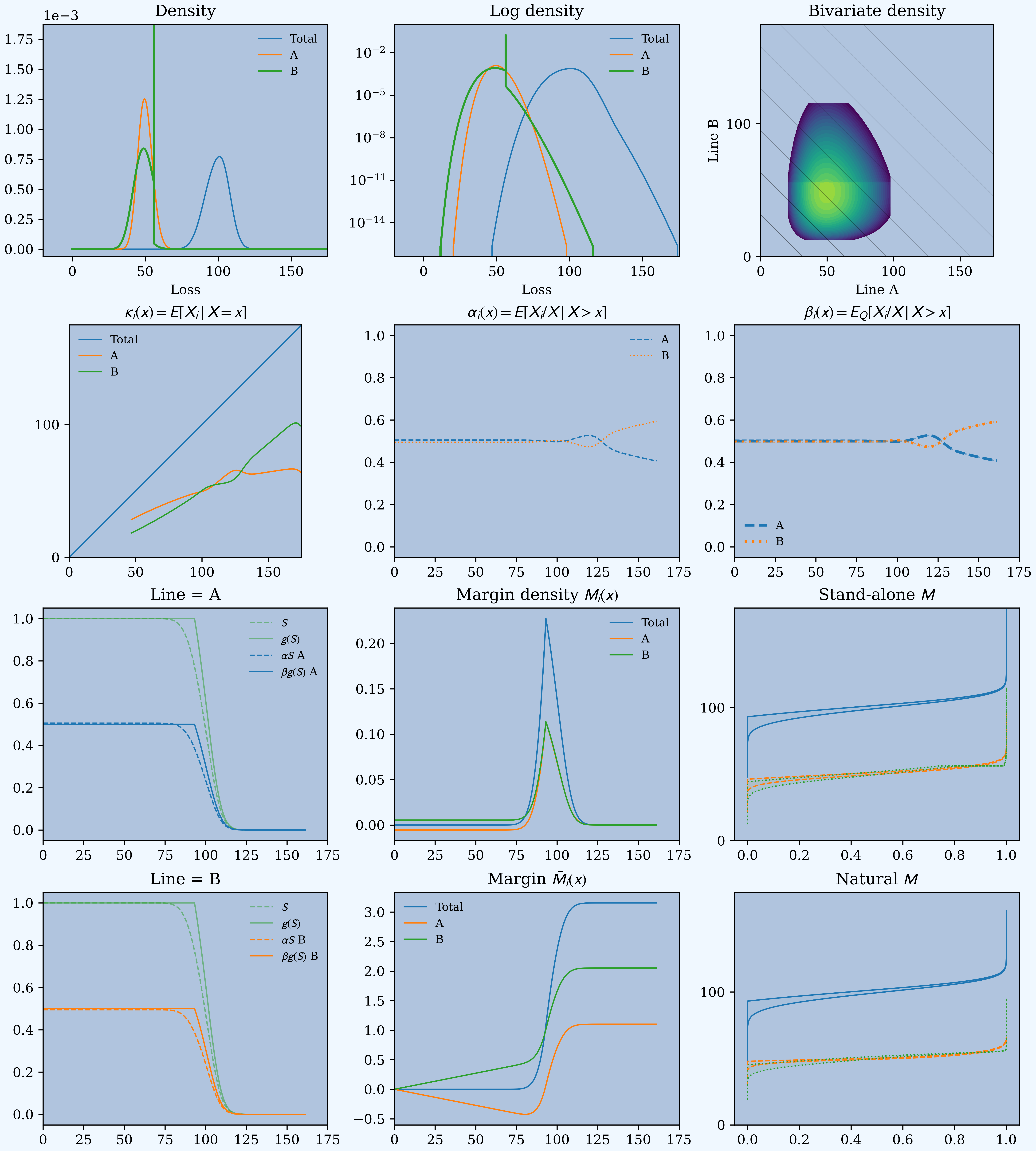
- Twelve-plot recapping densities and plotting κ. α, and β; premium and margin density by unit, cumulative margin by unit, and comparing the lifted natural allocation with stand-alone margins. Shown for gross and net losses, with different distortions.
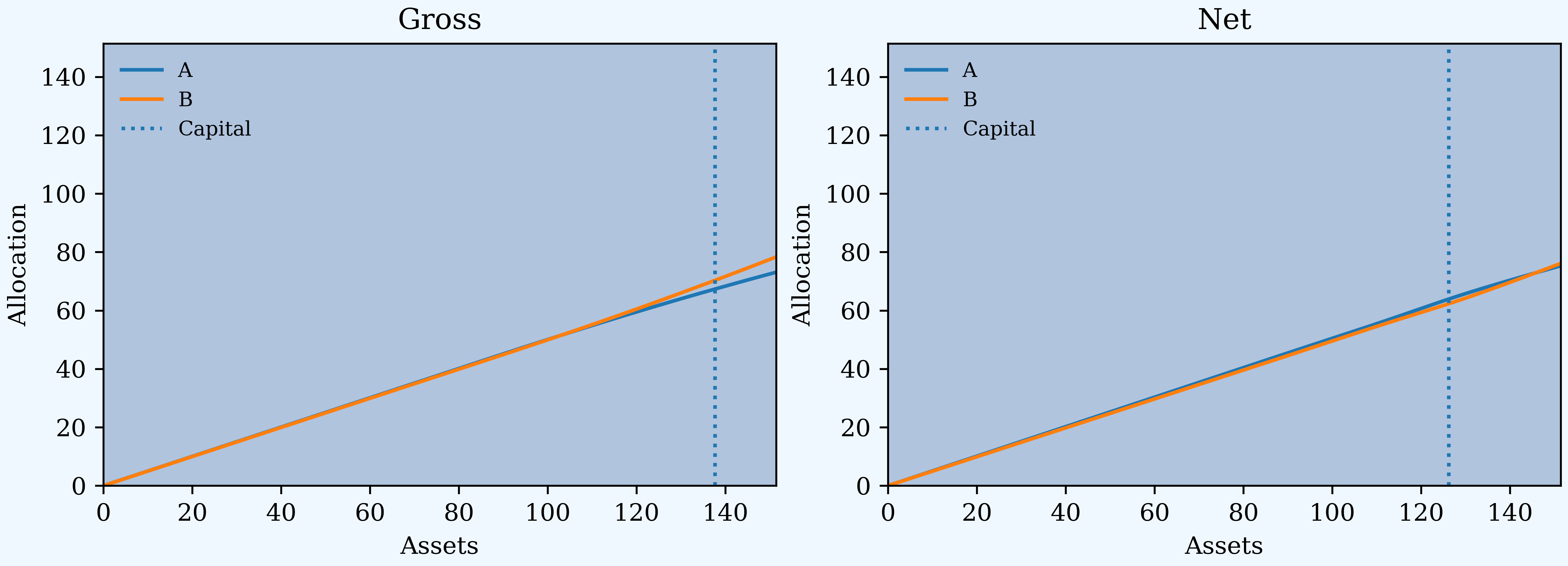
- Gross and net capital densities (marginal capital) as a function of assets.
- Allocated pricing and insurance statistics, gross and net, by unit by distortion, shown for CCoC, PH, Wang, Dual, TVaR, and the blend distortion.
- Conditional gross and net loss densities, κ, and distortion spectra by loss return period.
- Percentile layer of capital (PLC) allocated capital by asset level.
- Comparison of PLC and distortion pricing.


| Gross | Net | Ceded | ||||||
|---|---|---|---|---|---|---|---|---|
| line | A | B | Total | A | B | Total | Diff | |
| stat | Method | |||||||
| Loss | Expected Loss | 50.00 | 50.00 | 100.00 | 50.00 | 49.08 | 99.08 | 0.92 |
| Margin | Expected Loss | 1.71 | 1.71 | 3.42 | 1.24 | 1.22 | 2.46 | 0.96 |
| Dist ROE | 0.23 | 3.20 | 3.42 | 0.18 | 2.28 | 2.46 | 0.96 | |
| Dist PH | 1.00 | 2.42 | 3.42 | 1.37 | 1.39 | 2.76 | 0.66 | |
| Dist Wang | 1.04 | 2.39 | 3.42 | 1.28 | 1.63 | 2.90 | 0.52 | |
| Dist Dual | 1.07 | 2.36 | 3.42 | 1.18 | 1.85 | 3.03 | 0.39 | |
| Dist Tvar | 1.10 | 2.33 | 3.42 | 1.10 | 2.05 | 3.15 | 0.27 | |
| Dist Blend | 0.88 | 2.55 | 3.44 | 1.33 | 1.23 | 2.56 | 0.88 | |
| Premium | Expected Loss | 51.71 | 51.71 | 103.42 | 51.24 | 50.30 | 101.55 | 1.87 |
| Dist ROE | 50.23 | 53.20 | 103.42 | 50.18 | 51.37 | 101.55 | 1.87 | |
| Dist PH | 51.00 | 52.42 | 103.42 | 51.37 | 50.48 | 101.85 | 1.57 | |
| Dist Wang | 51.04 | 52.39 | 103.42 | 51.28 | 50.71 | 101.99 | 1.44 | |
| Dist Dual | 51.07 | 52.35 | 103.42 | 51.18 | 50.93 | 102.11 | 1.31 | |
| Dist Tvar | 51.10 | 52.33 | 103.42 | 51.10 | 51.14 | 102.24 | 1.18 | |
| Dist Blend | 50.88 | 52.55 | 103.44 | 51.33 | 50.31 | 101.65 | 1.79 | |
| Loss Ratio | Expected Loss | 0.97 | 0.97 | 0.97 | 0.98 | 0.98 | 0.98 | 0.49 |
| Dist ROE | 1.00 | 0.94 | 0.97 | 1.00 | 0.96 | 0.98 | 0.49 | |
| Dist PH | 0.98 | 0.95 | 0.97 | 0.97 | 0.97 | 0.97 | 0.58 | |
| Dist Wang | 0.98 | 0.95 | 0.97 | 0.98 | 0.97 | 0.97 | 0.64 | |
| Dist Dual | 0.98 | 0.96 | 0.97 | 0.98 | 0.96 | 0.97 | 0.70 | |
| Dist Tvar | 0.98 | 0.96 | 0.97 | 0.98 | 0.96 | 0.97 | 0.77 | |
| Dist Blend | 0.98 | 0.95 | 0.97 | 0.97 | 0.98 | 0.97 | 0.51 | |
| Capital | Expected Loss | 17.12 | 17.12 | 34.23 | 12.43 | 12.21 | 24.64 | 9.59 |
| Dist ROE | 2.25 | 31.98 | 34.23 | 1.82 | 22.82 | 24.64 | 9.59 | |
| Dist PH | 14.19 | 20.04 | 34.23 | 12.46 | 11.88 | 24.34 | 9.89 | |
| Dist Wang | 15.46 | 18.78 | 34.23 | 12.43 | 11.77 | 24.20 | 10.03 | |
| Dist Dual | 15.63 | 18.60 | 34.23 | 12.37 | 11.70 | 24.07 | 10.16 | |
| Dist Tvar | 15.66 | 18.57 | 34.23 | 12.31 | 11.64 | 23.95 | 10.28 | |
| Dist Blend | 10.90 | 23.32 | 34.22 | 12.58 | 11.96 | 24.54 | 9.68 | |
| Rate of Return | Expected Loss | 0.10 | 0.10 | 0.10 | 0.10 | 0.10 | 0.10 | 0.10 |
| Dist ROE | 0.10 | 0.10 | 0.10 | 0.10 | 0.10 | 0.10 | 0.10 | |
| Dist PH | 0.07 | 0.12 | 0.10 | 0.11 | 0.12 | 0.11 | 0.07 | |
| Dist Wang | 0.07 | 0.13 | 0.10 | 0.10 | 0.14 | 0.12 | 0.05 | |
| Dist Dual | 0.07 | 0.13 | 0.10 | 0.10 | 0.16 | 0.13 | 0.04 | |
| Dist Tvar | 0.07 | 0.13 | 0.10 | 0.09 | 0.18 | 0.13 | 0.03 | |
| Dist Blend | 0.08 | 0.11 | 0.10 | 0.11 | 0.10 | 0.10 | 0.09 | |
| Leverage | Expected Loss | 3.02 | 3.02 | 3.02 | 4.12 | 4.12 | 4.12 | 0.20 |
| Dist ROE | 22.34 | 1.66 | 3.02 | 27.64 | 2.25 | 4.12 | 0.20 | |
| Dist PH | 3.59 | 2.62 | 3.02 | 4.12 | 4.25 | 4.18 | 0.16 | |
| Dist Wang | 3.30 | 2.79 | 3.02 | 4.12 | 4.31 | 4.21 | 0.14 | |
| Dist Dual | 3.27 | 2.81 | 3.02 | 4.14 | 4.35 | 4.24 | 0.13 | |
| Dist Tvar | 3.26 | 2.82 | 3.02 | 4.15 | 4.39 | 4.27 | 0.12 | |
| Dist Blend | 4.67 | 2.25 | 3.02 | 4.08 | 4.21 | 4.14 | 0.19 | |
| Assets | Expected Loss | 68.83 | 68.83 | 137.66 | 63.68 | 62.51 | 126.19 | 11.47 |
| Dist ROE | 52.47 | 85.18 | 137.66 | 52.00 | 74.18 | 126.19 | 11.47 | |
| Dist PH | 65.19 | 72.46 | 137.66 | 63.83 | 62.35 | 126.19 | 11.47 | |
| Dist Wang | 66.49 | 71.16 | 137.66 | 63.71 | 62.48 | 126.19 | 11.47 | |
| Dist Dual | 66.70 | 70.96 | 137.66 | 63.55 | 62.63 | 126.19 | 11.47 | |
| Dist Tvar | 66.76 | 70.90 | 137.66 | 63.41 | 62.77 | 126.19 | 11.47 | |
| Dist Blend | 61.78 | 75.87 | 137.66 | 63.92 | 62.27 | 126.19 | 11.47 | |

| Gross | Net | Ceded | |||||
|---|---|---|---|---|---|---|---|
| line | A | B | Total | A | B | Total | Diff |
| Method | |||||||
| Expected Loss | 68.83 | 68.83 | 137.7 | 63.68 | 62.51 | 126.2 | 11.47 |
| Dist ROE | 52.47 | 85.18 | 137.7 | 52 | 74.18 | 126.2 | 11.47 |
| Dist PH | 65.19 | 72.46 | 137.7 | 63.83 | 62.35 | 126.2 | 11.47 |
| Dist Wang | 66.49 | 71.16 | 137.7 | 63.71 | 62.48 | 126.2 | 11.47 |
| Dist Dual | 66.7 | 70.96 | 137.7 | 63.55 | 62.63 | 126.2 | 11.47 |
| Dist Tvar | 66.76 | 70.9 | 137.7 | 63.41 | 62.77 | 126.2 | 11.47 |
| Dist Blend | 61.78 | 75.87 | 137.7 | 63.92 | 62.27 | 126.2 | 11.47 |
| PLC | 67.34 | 70.32 | 137.7 | 63.89 | 62.3 | 126.2 | 11.47 |
Created 2024-04-24 23:26:17.567386